workflowr

• Summary
• Checks
• Past versions

Last updated: 2024-09-10

Checks: 7 0

Knit directory: My_Project/

This reproducible R Markdown analysis was created with workflowr (version 1.7.1). The Checks tab describes the reproducibility checks that were applied when the results were created. The Past versions tab lists the development history.

---

R Markdown file: up-to-date

Great! Since the R Markdown file has been committed to the Git repository, you know the exact version of the code that produced these results.

Environment: empty

Great job! The global environment was empty. Objects defined in the global environment can affect the analysis in your R Markdown file in unknown ways. For reproduciblity it’s best to always run the code in an empty environment.

Seed: set.seed(20240905)

The command set.seed(20240905) was run prior to running the code in the R Markdown file. Setting a seed ensures that any results that rely on randomness, e.g. subsampling or permutations, are reproducible.

Session information: recorded

Great job! Recording the operating system, R version, and package versions is critical for reproducibility.

Cache: none

Nice! There were no cached chunks for this analysis, so you can be confident that you successfully produced the results during this run.

File paths: relative

Great job! Using relative paths to the files within your workflowr project makes it easier to run your code on other machines.

Repository version: 166be7f

Great! You are using Git for version control. Tracking code development and connecting the code version to the results is critical for reproducibility.

The results in this page were generated with repository version 166be7f. See the Past versions tab to see a history of the changes made to the R Markdown and HTML files.

Note that you need to be careful to ensure that all relevant files for the analysis have been committed to Git prior to generating the results (you can use wflow_publish or wflow_git_commit). workflowr only checks the R Markdown file, but you know if there are other scripts or data files that it depends on. Below is the status of the Git repository when the results were generated:

Ignored files:
    Ignored:    .Rhistory
    Ignored:    .Rproj.user/

Untracked files:
    Untracked:  .Rapp.history
    Untracked:  .gitignore
    Untracked:  Stats.Rmd
    Untracked:  Stats.html
    Untracked:  data/.DS_Store
    Untracked:  data/COADREAD.clin.merged.picked.txt
    Untracked:  data/COADREAD.rnaseqv2__illuminahiseq_rnaseqv2__unc_edu__Level_3__RSEM_genes_normalized__data.data.txt

Unstaged changes:
    Modified:   .DS_Store
    Modified:   analysis/.DS_Store
    Deleted:    myproject.zip

Note that any generated files, e.g. HTML, png, CSS, etc., are not included in this status report because it is ok for generated content to have uncommitted changes.

---

These are the previous versions of the repository in which changes were made to the R Markdown (analysis/EXAMPLE.Rmd) and HTML (docs/EXAMPLE.html) files. If you’ve configured a remote Git repository (see ?wflow_git_remote), click on the hyperlinks in the table below to view the files as they were in that past version.

File	Version	Author	Date	Message
html	c3ff74c	oliverdesousa	2024-09-10	Build site.
Rmd	5e763e5	oliverdesousa	2024-09-10	Start my new project

---

miRseq Analysis:

Analysing miRseq Gene Expression Data from a Colerectal Adenocarcinoma Cohort:

# install.packages("readxl")
# install.packages("readxl")
library(readxl)
library(KODAMA)
library(knitr)

Prepare Clinical Data:

# Read in Clinical Data:
coad=read.csv("data/COADREAD.clin.merged.picked.txt",sep="\t",check.names = FALSE)

# Set the first column as row names
rownames(coad) = coad[,1]
# Remove the first column as it is now used as row names
coad = coad[,-1]  
coad <- as.data.frame(coad) 

# Clean column names: replace dots with dashes & convert to uppercase
colnames(coad) = gsub("\\.", "-", toupper(colnames(coad)))

 # Transpose the dataframe so that rows become columns and vice versa
coad = t(coad) 

Prepare miRNA-seq expression data:

# Read RNA-seq expression data:
r = read.csv("data/COADREAD.rnaseqv2__illuminahiseq_rnaseqv2__unc_edu__Level_3__RSEM_genes_normalized__data.data.txt", sep = "\t", check.names = FALSE, row.names = 1)

# Remove the first row:
r = r[-1,]

# Convert expression data to numeric matrix format
temp = matrix(as.numeric(as.matrix(r)), ncol=ncol(r))

# Assign original column names to the matrix
colnames(temp) = colnames(r)  
# Assign original row names to the matrix
rownames(temp) = rownames(r)  
RNA = temp  

# Transpose the matrix so that genes are rows and samples are columns
RNA = t(RNA)  

Extract patient and tissue information from column names:

tcgaID = list()
 # Extract sample ID
tcgaID$sample.ID <- substr(colnames(r), 1, 16)
# Extract patient ID
tcgaID$patient <- substr(colnames(r), 1, 12)  
# Extract tissue type
tcgaID$tissue <- substr(colnames(r), 14, 16)  

tcgaID = as.data.frame(tcgaID)  

Select Primary Solid Tumor tissue data (“01A”):

tcgaID.sel = tcgaID[tcgaID$tissue == "01A", ]

# Subset the RNA expression data to match selected samples
RNA.sel = RNA[tcgaID$tissue == "01A", ]

Intersect patient IDs between clinical and RNA data:

sel = intersect(tcgaID.sel$patient, rownames(coad))
# Subset the clinical data to include only selected patients:
coad.sel = coad[sel, ]
# Assign patient IDs as row names to the RNA data:
rownames(RNA.sel) = tcgaID.sel$patient
# Subset the RNA data to include only selected patients
RNA.sel = RNA.sel[sel, ]

Prepare labels for pathology stages:

• Classify stages t1, t2, & t3 as “low”

• Classify stages t4, t4a, & t4b as “high”

• Convert any tis stages to NA

labels = coad.sel[, "pathology_T_stage"]

labels[labels %in% c("t1", "t2", "t3")] = "low"

labels[labels %in% c("t4", "t4a", "t4b")] = "high"

labels[labels == "tis"] = NA

Log Transform the expression data for our selected gene CXCL2:

CXCL2 <- log(1 + RNA.sel[, "CXCL2|2920"])

Boxplot to visualize the distribution of log transformed gene expression by pathology stage:

boxplot(CXCL2 ~ labels, main = "Expression of CXCL2 by Pathology Stage",
        xlab = "Pathology Stage",
        ylab = "Log Transformed Expression",
        col = c("lightyellow", "sandybrown"))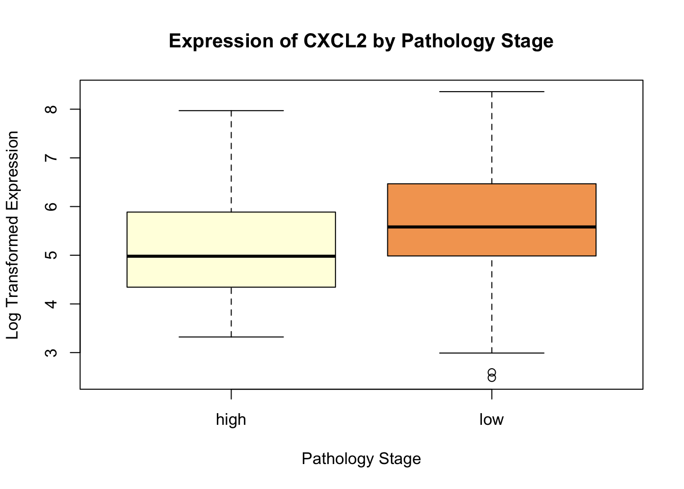 

Past versions of unnamed-chunk-9-1.png

Version	Author	Date
c3ff74c	oliverdesousa	2024-09-10

Perform Wilcoxon rank-sum test to compare gene expression between “low” and “high” stages:

CXCL2_W <- wilcox.test(CXCL2 ~ labels)
CXCL2_W

    Wilcoxon rank sum test with continuity correction

data:  CXCL2 by labels
W = 5357, p-value = 0.0007265
alternative hypothesis: true location shift is not equal to 0

Now, we log transform expression data for three other genes:

CXCL3 <- log(1 + RNA.sel[, "CXCL3|2921"])
GPX2 <- log(1 + RNA.sel[, "GPX2|2877"])
LCN2 <- log(1 + RNA.sel[, "LCN2|3934"])

Visualize the log transformed gene expression by pathology stage for all four genes:

par(mfrow = c(1, 4))
ylim_range <- c(2, 12)

# CXCL2 boxplot:
boxplot(CXCL2 ~ labels, main = "CXCL2",
        xlab = "Pathology Stage",
        ylab = "Log Transformed Expression",
        col = c("lightyellow", "sandybrown"),
        ylim = ylim_range) 

# GPX2 boxplot:
boxplot(GPX2~ labels, 
        main = "GPX2",
        xlab = "Pathology Stage",
        ylab = "Log Transformed Expression",
        col = c("lightblue", "lightcoral"),
        ylim = ylim_range)  # Specify colors for each box

# CXCL3 boxplot:
boxplot(CXCL3 ~ labels, 
        main = "CXCL3",
        xlab = "Pathology Stage",
        ylab = "Log Transformed Expression",
        col = c("lightgreen", "lightgoldenrod"),
        ylim = ylim_range)  # Specify colors for each box

# LCN2 boxplot:
boxplot(LCN2 ~ labels, 
        main = "LCN2",
        xlab = "Pathology Stage",
        ylab = "Log Transformed Expression",
        col = c("lightpink", "lightsteelblue"),
        ylim = ylim_range)  # Specify colors for each box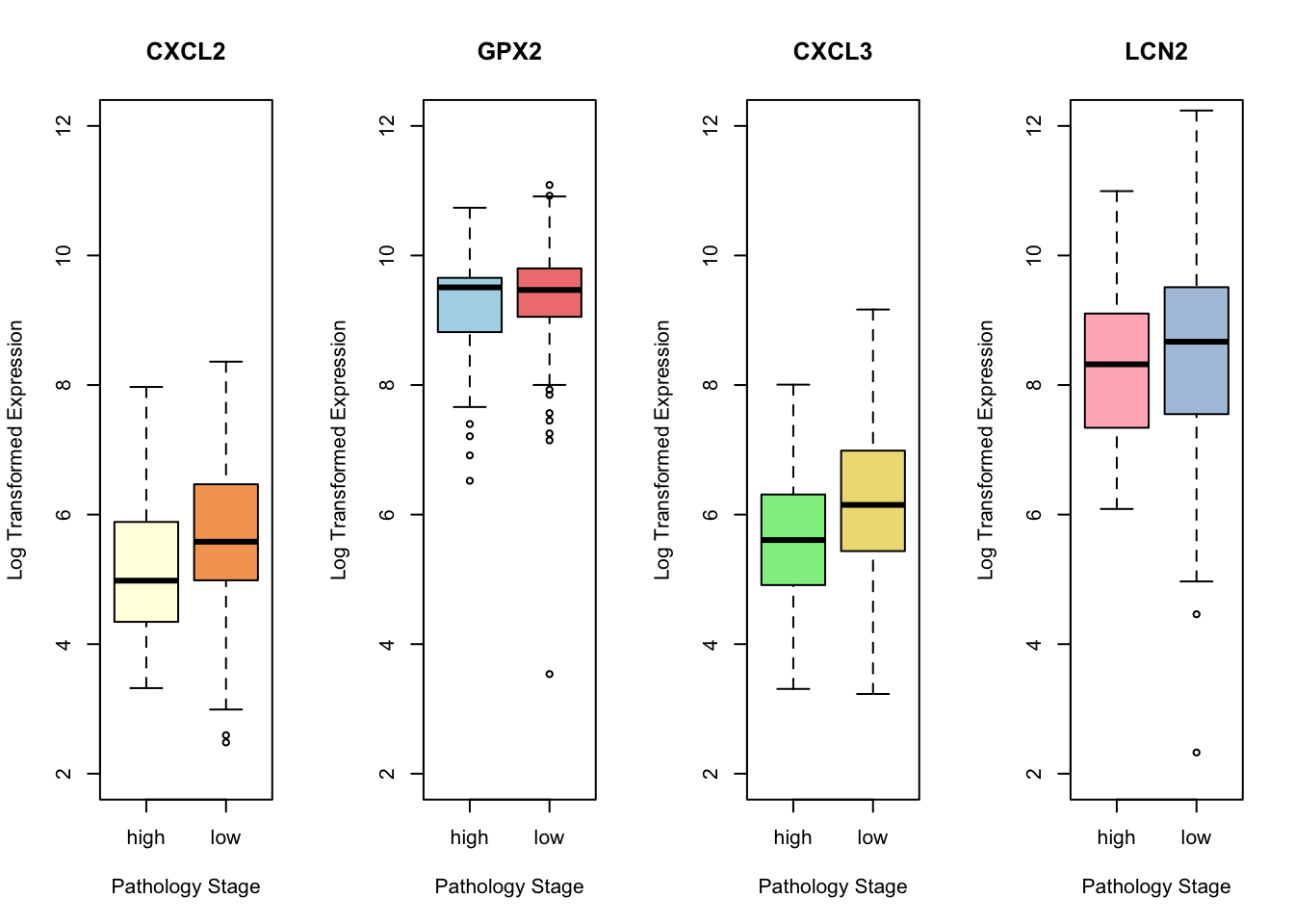

Past versions of unnamed-chunk-12-1.png

Version	Author	Date
c3ff74c	oliverdesousa	2024-09-10

par(mfrow = c(1, 1))

Perform Wilcoxon rank-sum test to compare gene expression between “low” and “high” stages for the three new genes:

# LCN2 Gene:
LCN2_W <- wilcox.test(LCN2~ labels)
# CXCL3 Gene:
CXCL3_W <- wilcox.test(CXCL3 ~ labels)
# GPX2 Gene:
GPX2_W <- wilcox.test(GPX2 ~ labels)

Now lets compare their output from the Wilcoxon rank-sum test:

results <- data.frame(
  Gene = c("LCN2", "CXCL3", "GPX2", "CXCL2"),
  Test_Statistic = c(LCN2_W$statistic, CXCL3_W$statistic, GPX2_W$statistic, CXCL2_W$statistic),
  P_Value = c(LCN2_W$p.value, CXCL3_W$p.value, GPX2_W$p.value, CXCL2_W$p.value),
  stringsAsFactors = FALSE
)

kable(results, digits = 4)

Gene	Test_Statistic	P_Value
LCN2	6916	0.2666
CXCL3	5119	0.0002
GPX2	7083	0.3854
CXCL2	5357	0.0007

Interpretation:

• CXCL2 (0.0007) and CXCL3 (0.0002) showed significant differences in gene expression between high and low pathology stages, with p-values < 0.05.

• This result suggests that these genes could be important in distinguishing between different stages of the disease and warrants further investigation into their roles and potential as biomarkers or therapeutic targets.

Session information

sessionInfo()

R version 4.4.1 (2024-06-14)
Platform: aarch64-apple-darwin20
Running under: macOS Sonoma 14.6.1

Matrix products: default
BLAS:   /Library/Frameworks/R.framework/Versions/4.4-arm64/Resources/lib/libRblas.0.dylib 
LAPACK: /Library/Frameworks/R.framework/Versions/4.4-arm64/Resources/lib/libRlapack.dylib;  LAPACK version 3.12.0

locale:
[1] en_US.UTF-8/en_US.UTF-8/en_US.UTF-8/C/en_US.UTF-8/en_US.UTF-8

time zone: Africa/Johannesburg
tzcode source: internal

attached base packages:
[1] stats     graphics  grDevices utils     datasets  methods   base     

other attached packages:
[1] knitr_1.48     KODAMA_3.1     umap_0.2.10.0  Rtsne_0.17     minerva_1.5.10
[6] readxl_1.4.3  

loaded via a namespace (and not attached):
 [1] Matrix_1.7-0      jsonlite_1.8.8    highr_0.11        compiler_4.4.1   
 [5] promises_1.3.0    Rcpp_1.0.13       stringr_1.5.1     git2r_0.33.0     
 [9] parallel_4.4.1    later_1.3.2       jquerylib_0.1.4   png_0.1-8        
[13] yaml_2.3.10       fastmap_1.2.0     reticulate_1.38.0 lattice_0.22-6   
[17] R6_2.5.1          workflowr_1.7.1   tibble_3.2.1      openssl_2.2.1    
[21] rprojroot_2.0.4   bslib_0.8.0       pillar_1.9.0      rlang_1.1.4      
[25] utf8_1.2.4        cachem_1.1.0      stringi_1.8.4     httpuv_1.6.15    
[29] xfun_0.47         fs_1.6.4          sass_0.4.9        cli_3.6.3        
[33] magrittr_2.0.3    grid_4.4.1        digest_0.6.37     rstudioapi_0.16.0
[37] askpass_1.2.0     lifecycle_1.0.4   vctrs_0.6.5       RSpectra_0.16-2  
[41] evaluate_0.24.0   glue_1.7.0        whisker_0.4.1     cellranger_1.1.0 
[45] fansi_1.0.6       rmarkdown_2.28    tools_4.4.1       pkgconfig_2.0.3  
[49] htmltools_0.5.8.1